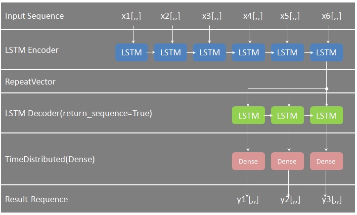
株価、為替、天気、動画など時系列データの予測でよく使われるディープラーニングの代表的手法RNN(再帰型ニューラルネットワーク)の拡張バージョンに、LSTM(Long short-term memory)と呼ばれるモデルがある。今回はLSTM Many to Oneモデルを実装して、複数銘柄(例:10銘柄)の株価から翌日の上がる株を探ってみる。
環境
keras 2.2.5 LSTM
Google Colab CPU/GPU/TPU
Ubuntu 18.04.3 LTS
Python 3.6.8
Numpy 1.17.3
Pandas 0.25.2
sklearn 0.21.3
実装
Many-to-Oneモデルの例として、以下2銘柄から翌日の上がる株を探る。
# -*- coding: utf-8 -*-
import numpy
import pandas
import matplotlib.pyplot as plt
from sklearn import preprocessing
from keras.models import Sequential
from keras.layers.core import Dense, Activation
from keras.layers.recurrent import LSTM
class Predict:
def __init__(self):
self.length_of_sequences = 10
self.in_out_neurons = 1
self.hidden_neurons = 300
self.batch_size = 32
self.epochs = 100
self.percentage = 0.8
# データ用意
def load_data(self, data, n_prev):
x, y = [], []
for i in range(len(data) - n_prev):
x.append(data.iloc[i:(i+n_prev)].values)
y.append(data.iloc[i+n_prev].values)
X = numpy.array(x)
Y = numpy.array(y)
return X, Y
# モデル作成
def create_model(self) :
Model = Sequential()
Model.add(LSTM(self.hidden_neurons, batch_input_shape=(None, self.length_of_sequences, self.in_out_neurons), return_sequences=False))
Model.add(Dense(self.in_out_neurons))
Model.add(Activation("linear"))
Model.compile(loss="mape", optimizer="adam")
return Model
# 学習
def train(self, x_train, y_train) :
Model = self.create_model()
Model.fit(x_train, y_train, self.batch_size, self.epochs)
return Model
if __name__ == "__main__":
predict = Predict()
nstocks = 2;
# 銘柄毎に学習、予測、表示
for istock in range(1, nstocks + 1):
# データ準備
data = None
data = pandas.read_csv('/content/drive/My Drive/LSTM/csv/' + str(istock) + '_stock_price.csv')
data.columns = ['date', 'open', 'high', 'low', 'close']
data['date'] = pandas.to_datetime(data['date'], format='%Y-%m-%d')
# 終値のデータを標準化
data['close'] = preprocessing.scale(data['close'])
data = data.sort_values(by='date')
data = data.reset_index(drop=True)
data = data.loc[:, ['date', 'close']]
# 割合で学習、試験データ分割
split_pos = int(len(data) * predict.percentage)
x_train, y_train = predict.load_data(data[['close']].iloc[0:split_pos], predict.length_of_sequences)
x_test, y_test = predict.load_data(data[['close']].iloc[split_pos:], predict.length_of_sequences)
# 学習
model = predict.train(x_train, y_train)
# 試験
predicted = model.predict(x_test)
result = pandas.DataFrame(predicted)
result.columns = [str(istock) + '_predict']
result[str(istock) + '_actual'] = y_test
# 表示
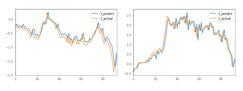
result.plot()
plt.show()
# 翌日株価比較
current = result.iloc[-1][str(istock) + '_actual']
predictable = result.iloc[-1][str(istock) + '_predict']
if (predictable - actual) > 0:
print(f'{istock} stock price of the next day INcreases: {predictable-actual:.2f}, predictable:{predictable:.2f}, current:{current:.2f}')
else:
print(f'{istock} stock price of the next day DEcreases: {actual-predictable:.2f}, predictable:{predictable:.2f}, current:{current:.2f}')