概要
kd-tree(k-dimensions tree)はk次元空間の分割を表す二分木である。kd-treeの構築は、座標軸に垂直な超平面でk次元空間を連続的に分割して、一連のk次元超長方形領域を形成する。 kd-treeの各ノードは、k次元の超長方形領域に対応する。kd-treeを使用すると、一部のインスタンスとの計算はしないため、計算量が削減される。よって、kd-treeは早く探索できるようにインスタンスポイントをk次元空間に格納するツリー型のデータ構造である。それで新しいインスタンスのクラス(属するクラス)をkd-treeによる判明する最近傍探索のアルゴリズムは以下のとおり。
【step1】k次元データセットで最大の分散をもつ次元xを選択し、次に中央値mを次元の中間点として選択してデータセットを分割し、2つのサブセットを取得する。
【step2】2つのサブセットに対してステップstep1のプロセスを繰り返して、すべてのサブセットが再分割できなくなるまで繰り返す。
【step3】step1とstep2で根から葉っぱまで木ができてしまう。
【step4】根から葉っぱまで、あるルール「\(x \lt m\)→左枝、\(x \geq m\)→右枝」で新しいインスタンスに最も近いインスタンス(葉っぱ、ノード)をみつける。
【step5】step4の葉っぱから、逆方向で根まで遡って、step4よりもっと近いインスタンスがあるか探索する。要するに、新しいインスタンスにもっとも近い既存インスタンスをみつける。
【step6】step4またはstep5でみつけたもっとも近い既存インスタンスのクラスは結果となる。
実装の例
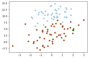
下図から、グリーンポイント[2, 4.5]に最近傍ポイントを探索する。
# -*- coding: utf-8 -*-
import numpy as np
import matplotlib.pyplot as plt
#from time import time

#
# load data from dataset file.
#
def load_data(fileName):
    data_mat = []
    with open(fileName) as fd:
        for line in fd.readlines():
            data = line.strip().split()
            data = [float(item) for item in data]
            data_mat.append(data)
    data_mat = np.array(data_mat)
    label = data_mat[:, 2]
    data_mat = data_mat[:, :2]
    return data_mat, label
#
# create a tree for dataset.
#
def create_kdtree(dataset, depth):
    n = np.shape(dataset)[0]
    tree_node = {}
    if n == 0:
        return None
    else:
        n, m = np.shape(dataset)
        split_axis = depth % m
        depth += 1
        tree_node['split'] = split_axis
        dataset = sorted(dataset, key=lambda a: a[split_axis])
        num = n // 2
        tree_node['median'] = dataset[num]
        tree_node['left'] = create_kdtree(dataset[:num], depth)
        tree_node['right'] = create_kdtree(dataset[num + 1:], depth)
        return tree_node
#
# search k near points on the tree.
#
def search_kdtree(tree, data):
    k = len(data)
    if tree is None:
        return [0] * k, float('inf')
    split_axis = tree['split']
    median_point = tree['median']
    if data[split_axis] <= median_point[split_axis]:
        nearest_point, nearest_distance = search_kdtree(tree['left'], data)
    else:
        nearest_point, nearest_distance = search_kdtree(tree['right'], data)

    # the distance between data to current point.
    now_distance = np.linalg.norm(data - median_point)
    if now_distance < nearest_distance:
        nearest_distance = now_distance
        nearest_point = median_point.copy()

    # the distance between hyperplane.
    split_distance = abs(data[split_axis] - median_point[split_axis])
    if split_distance > nearest_distance:
        return nearest_point, nearest_distance
    else:
        if data[split_axis] <= median_point[split_axis]:
            next_tree = tree['right']
        else:
            next_tree = tree['left']
        near_point, near_distance = search_kdtree(next_tree, data)
        if near_distance < nearest_distance:
            nearest_distance = near_distance
            nearest_point = near_point.copy()
        return nearest_point, nearest_distance
#
# main.
#
if __name__ == '__main__':
    data_mat, label = load_data('/content/drive/My Drive/Colab Notebooks/Machine_Learning/kd_tree/dataset.txt')
    fig = plt.figure(0)
    ax = fig.add_subplot(111)
    ax.scatter(data_mat[:, 0], data_mat[:, 1], c=label, cmap=plt.cm.Paired)

    new_point = [2, 4.5]
    kdtree = create_kdtree(data_mat, 0)
    print(kdtree)
    #start = time()
    nearest_point, near_dis= search_kdtree(kdtree, new_point)
    #print(time()-start)
    ax.scatter(new_point[0], new_point[1], c='g', s=50)
    ax.scatter(nearest_point[0], nearest_point[1], c='r', s=50)
    plt.show()
ソースコード→https://github.com/soarbear/Machine_Learning/tree/master/kd_tree
結果

kd-treeが小さい(例えば\(k=20\))場合、アルゴリズムの探索効率はkNNより非常に高くなる。ただし、データの次元が増えると(例えば、\(k≥100\))、探索効率が急速に低下する。データセットの次元がkであると仮定すると、効率的な探索を実現するために、データサイズNが、\(N >> 2^k\)を満たすことが必要である。kd-treeで高次元データにも適用できるように、Jeffrey S. BeisとDavid G. Loweは、改善されたアルゴリズムKd-tree with BBF(Best Bin First)の提案に貢献した。ある探索精度を確保するという前提で探索を高速化するようになる。
参考文献
「Machine Learning in Action」、Peter Harrington氏
ロボット・ドローン部品お探しなら![]()